
この「羅針盤の示す先」カテゴリーでは、有機化学の教科書などで見たことのある基本的な内容について、オープンソースの計算プログラムを用いた計算の結果を公開していきます。
すでに知られていたり、論文で公表するほどではない些細な内容になるかもしれませんが、有機化学や計算化学を学んでいる方に少しでも役に立てばと思っています。
有償プログラムは計算結果の公開に制限があることも多いため、このカテゴリーではPsi4やGromacsといったオープンソースのプログラムを用います。
インプットファイルやスクリプトについても合わせて紹介しますので、これらのプログラムを用いる方の参考になれば幸いです。
・分子力場とはどのようなものか
・分子力場計算と量子化学計算の結果はどの程度異なるのか
・Psi4を用いたrelaxed scanのスクリプト
分子力場計算とは
Schrödinger方程式やKohn–Sham方程式が基盤となっている量子化学(QM)計算は、その計算コストから大きな分子への適用には限界があります。
このような観点から、原子を「球」、結合を「バネ」のように見立てた分子力場を使った分子力場(MM)計算が開発されてきました。
よく使われる力場として
・CHARMM力場
・AMBER力場
・MM2力場
・OPLS力場
などがあります。
電子が作る化学結合を単純なバネとして表現してよいのか疑問に思う方もいるかもしれません。
今回の記事ではCHARMM36m力場とDFT計算を比較してどれくらいの違いが生じるのかを検証します。
分子力場の基礎的な解説も含んでいるので、分子動力学シミュレーションを学び始めている方にも役立つと内容かと思います。
今回の計算対象
分子力場ではバネの定義が必要ですが、分子を定義するためには
・結合距離 (bond)
・角度 (bend, angle)
・二面角 (dihedral)
に対する力場(バネ)の定義が必要です。
これら3つのデータを調べるため今回は
ethane(CH3CH3)のC-H結合やC-C結合について調べてみました。
計算条件
計算条件は
量子化学(QM):ωB97X-D/Def2-SV(P)
分子力場(MM):CHARMM36
としました。
量子化学計算はPsi4を用いて行いました。
Psi4の使い方については
化学の新しいカタチ:【まとめ】Psi4の使い方
でよくまとめられています。
参考にしたCHARMM力場については
CHARMM-GUIのLesson 3に詳細が記載されています。
今回はこのページから結合や角度、二面角のパラメーターをとってきて、表計算ソフトを使ってエネルギーを計算しています。(つまり、MM計算については計算化学用の特別なプログラムは使用していません。)
結合(bond)パラメーターの比較
CHARMM力場における結合パラメーター
CHARMM-GUIのLesson 3では、プロパンのパラメーターが説明されていますが、エタンとほとんど同じですので、こちらを用います。
CHARMM力場における結合(bond)は、フックの法則に従う形で以下のように定義されています。
\[V_{bond}\,=\,K_b(b-b_0)^2・・・\rm{(1)}\]
ここで、\(b_0\)は結合の自然長を表し、ポテンシャル\(V_{bond} \)は結合長が自然長からズレた際にどの程度エネルギーが変化するかを表します。
ethaneのC-H結合については以下のようにパラメーターが設定されています。
(!以降はコメントです。)
atom-type   atom-type   Kb   b0
CG331  HGA3    322.00     1.1110 ! PROT alkane update, adm jr., 3/2/92
つまり、
\(K_b\,=\,322.00\,kcal/mol·\rm{Å}^2\)
\(b_0\,=\,1.1110\,\rm{Å}\)
と設定されているということです。
このパラメーター定義される二次関数(1)をC-Hの結合長\(b\)に対してプロットしてみます。
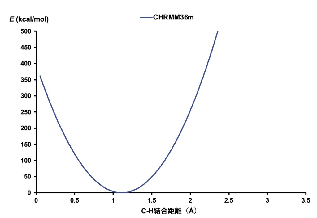
二次関数なので当然ですが、下に凸の放物線になります。
C-H結合に対するrelaxed scan (DFT計算)
次に、DFT計算により、エタンのC-H結合に対するrelaxed scanを行った結果を示します。
Psi4ではrelaxed scan行うためのオプションが定義されていないため、制約付き最適化応用する形で自分でスクリプトを書く必要がありますが、基本的には
①指定した座標(距離・角度・二面角)を初期値に固定した構造最適化
②構造最適化された構造を新しい入力構造として、指定した座標を少し変化させて再度構造最適化
③得られた最適化構造を次の段階の初期構造として上記サイクルを繰り返す
という流れをpythonのループ処理で行ってあげればよいです。
スクリプトは本記事の後半に公開しておきます。
計算したい分子の3次元構造を変えれば動くようになっていると思いますので、そのまま使っても良いですし、もっと良いスクリプトに変えてもらっても構いません。
このスクリプトはこのあと出てくる角度や二面角のrelaxed scanのスクリプトのように、分子を二分割して距離を変更するようにするとよりよいスクリプトになります。(今回はこれでよいかなと思っています。)
ethaneに対して計算を行い、C-H結合長\(b\)に対してプロットした結果が以下の図です。
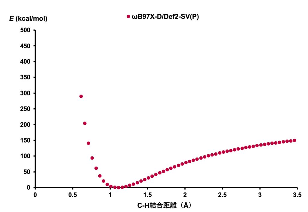
有機化学の教科書で見たことのあるような形をしていますね。
力場計算とDFT計算の比較(bond)
先ほどのグラフ同士を重ねてみます。
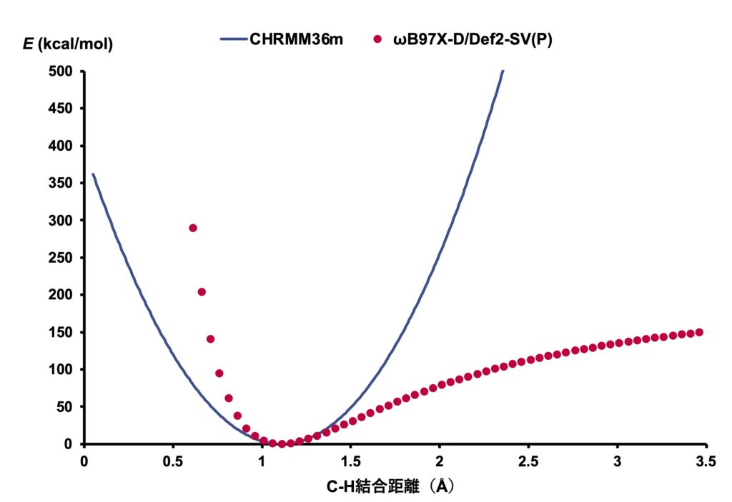
0.9 Å〜1.4 Åの間では許容できる程度の誤差ですが、それ以外の領域では大きく乖離していますね。
この結果から、結合パラメーターについては、自然長(約1.1 Å)近傍は量子化学と遜色ないエネルギーを与えるといって良さそうです。
特に、極小の位置はほとんど同一なので、安定構造に与える影響は小さいと考えられます。
一方で、結合が乖離するような距離になると誤差が大きいことから、遷移状態の計算には分子力場計算が適用できないこともわかります。
角度(bend)パラメーターの比較
CHARMM力場における角度パラメーター
CHARMM-GUIのLesson 3では、角度についても定義式(2)の記載があります。
\[V\,=\,V_{angle}\,+\,V_{Urey-Bradley}・・・\rm{(2)}\]
右辺第一項は、以下の式で表されるように、角度\(θ\)を変数とするちょうつがい型のバネモデルです。
\[V_{angle}\,=\,K_θ(θ-θ_0)^2\]
右辺第二項は、以下の式で表現できるUrey-Bradleyポテンシャルで、A-B-Cという三原子の並び(\(∠ABC = θ\))において、AとCの距離\(S\)に対するバネです。(A-C間にバネがあるイメージ)
\[V_{Urey-Bradley}\,=\,K_{UB}(S-S_0)^2\]
ethaneについてはC-C-Hの角度パラメーターが以下のように定義されています。
atom-type atom-type atom-type    Kθ   θ0   KUB   S0
CG331  CG321  HGA2     34.60    110.10   22.53   2.17900 !  PROT alkane update, adm jr., 3/2/92
結合パラメーターと同様ですが
\(K_θ\,=\,34.60\,kcal/mol·rad^2\)
\(θ_0\,=\,110.10°\)
\(K_{UB}\,=\,22.53\,kcal/mol·\rm{Å}^2\)
\(S_0\,=\,2.17900\,\rm{Å}\)
という定数が設定されています。
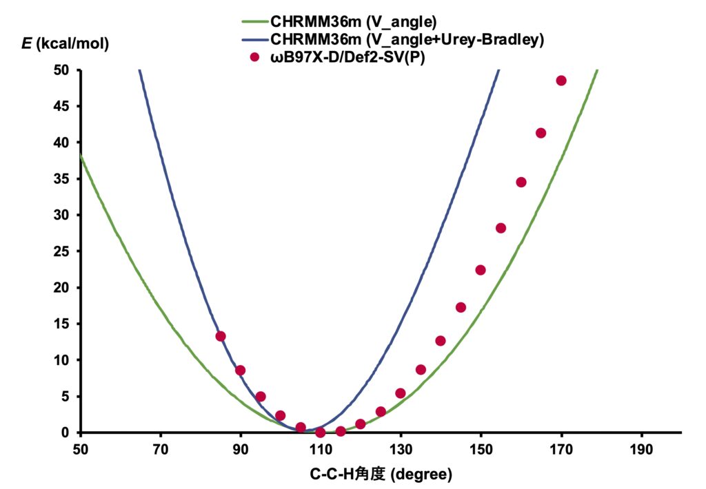
式(2)に上記定数を代入してプロットすると以下の青線のようになります。
(C-H結合長を1.11 Å、C-C結合長を1.53 Åに固定して\(S\)を求めています。)
なお、Urey-Bradleyポテンシャルを加えないと、緑色の曲線になります。
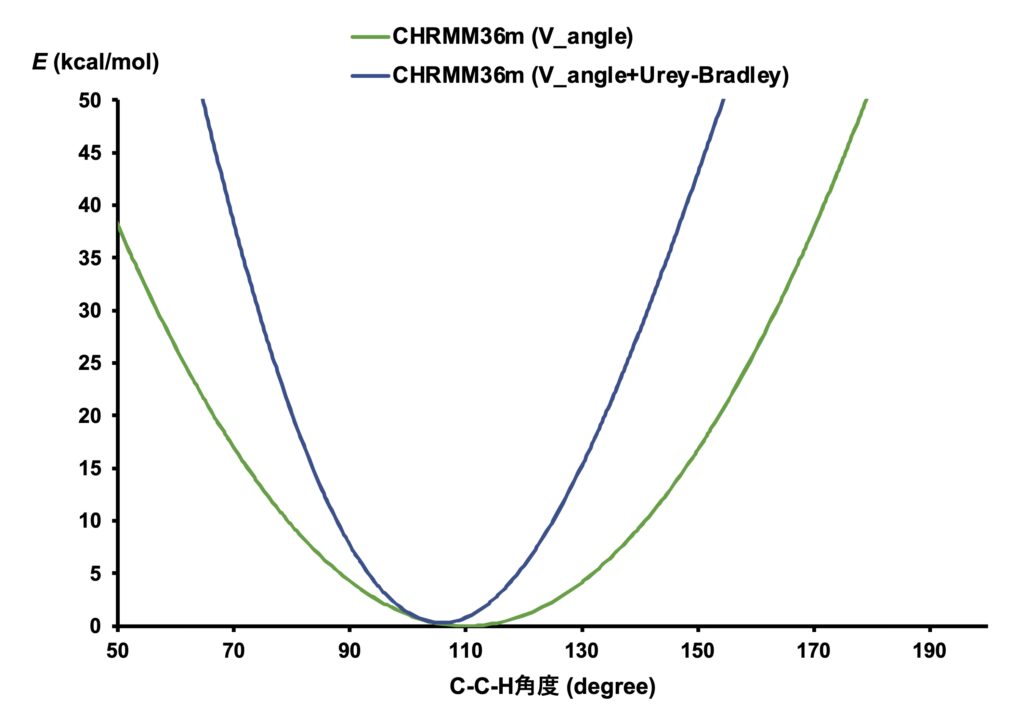
1つの二次関数のみで表現された緑色の曲線と比べて、青色の曲線はUrey-Bradleyポテンシャルを加えた分、左右非対称になっています。
これがDFT計算の結果と比較してどうなのかを見ていきましょう。
C-C-H角度に対するrelaxed scan・MM計算との比較
角度に対してrelaxed scanを行う場合は、
角度を固定した構造最適化→角度の変更→角度を固定した構造最適化
を繰り返すことになりますが、角度を変更するところの処理を少し工夫する必要があります。
以下の図を見てください。一原子(今回は左の炭素)のみを動かして、C-C-Hがなす角度を変えようとするとと、その炭素に結合しているC-H結合の長さが変わってしまい、全体としていびつな構造になってしまいます。
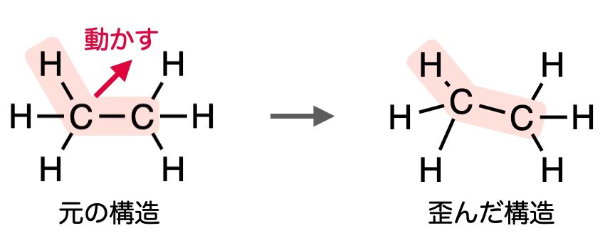
これをなんとかするため、分子を2つに分けてから角度を変化させます。
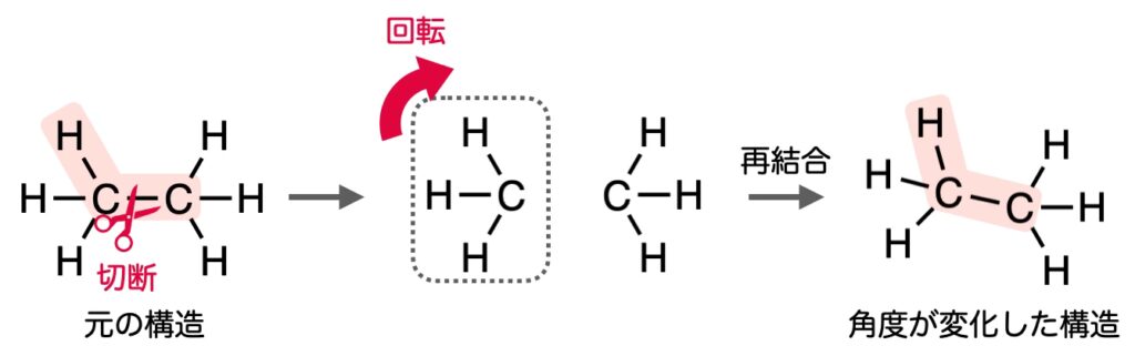
例えば以下の図のように、C-C結合で切断した左側のみの構造を考え、その部分全体を回転・移動してあげると、C-H結合長を保ったまま、角度の変更ができます。
スクリプトは記事後半に公開しておきますが、こちらのスクリプトで角度とエネルギーの関係を計算した結果が次の図です。(角度を小さくする方向は構造最適化に失敗することが多く、データがあまりありません。計算設定を変えればうまくいくのだろうと思っていますがこの記事ではこれで十分と判断しました。)
(2024/11/16追記)
結合距離のrelaxed scanのスクリプトも上と同様の仕組みのものに修正しました。
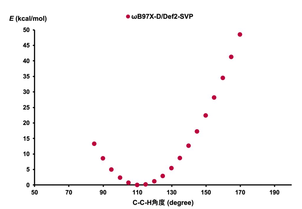
これを表計算ソフトで求めた分子力場計算のポテンシャルと重ねると、Urey-Bradleyポテンシャルを含む青色の曲線では、極小から大きい方向に離れるにつれて乖離が大きいことがわかります。
Urey-Bradleyポテンシャルを加えない場合は角度が大きい領域ではDFT計算とより一致しますが、角度が小さくなる方向については差が大きいですね。
両者のバランスを取って、このようなポテンシャルとなっているということなのでしょう。
結合パラメーターと比較して、極小の位置のズレが大きいのも少し気になりますね。
二面角(dihedral)パラメーターの比較
CHARMM力場における二面角パラメーターとDFT計算の比較
最後は二面角パラメーターです。
こちらも、CHARMM-GUIのLesson 3に記載があり、二面角\(χ\)について以下の定義式となっています。
\[V_{dihedral}\,=\,K_χ(1+cos(nχ-δ))・・・\rm{(3)}\]
ここで\(n\)はsinカーブの周期を決める定数(整数)、\(δ\)は位相のズレを表す値です。
有機化合物の構造特性から、位相のズレは0°か180°がほとんどです。
ethaneのH-C-C-H二面角については以下のパラメーターが設定されています。
atom-type atom-type atom-type atom-type    Kχ   n   δ
HGA2   CG321  CG331  HGA3       0.1600  3     0.00 ! PROT rotation barrier in Ethane (SF)
\(K_χ\,=\,0.1600\,kcal/mol\)
\(n\,=\,3\)
\(δ\,=\,0°\)
となります。
\(n = 3\)なので、120°周期のサインカーブが描かれることになります。
角度と同様に分子をC-C結合で2つに分割してから二面角を変更する方法でethaneのrelaxed scanを行いました。(スクリプトはこちら)
この結果を式(3)のポテンシャルと比べてみましょう。
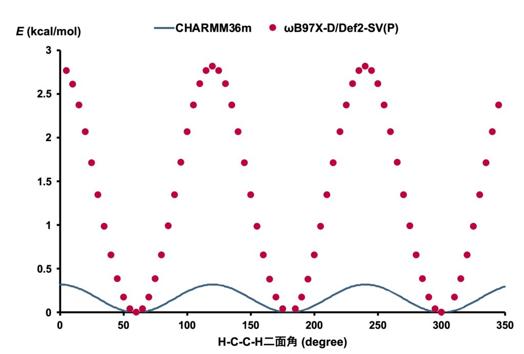
形は似ていますが、値が全然違いますね。
DFT計算ではethane全体のエネルギーを計算していますが、CHARMM力場のポテンシャルでは一組のH-C-C-Hのエネルギーしか計算していないのが原因です。
正しく計算するためには、水素6個(Me基の3H×Me基の3Hの組み合わせ)を考える必要があります。
厳密に考えるのであれば、あるHに対して、120°異なる二面角のHが2つ存在するのですが、今考えているポテンシャルでは\(n = 3\)で、周期と一致してくれるので、単純に3×3 = 9倍すればよいです。
ポテンシャルを9倍してからDFT計算の結果を重ねると
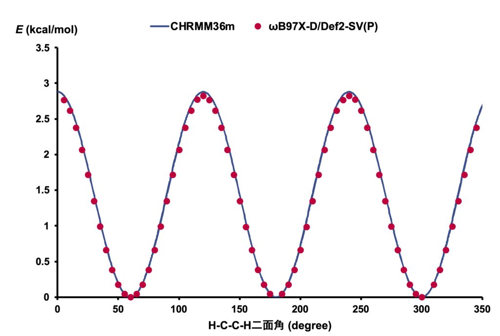
このようにほとんど一致する結果が得られました。
角度や結合長のような二次関数ではなく、三角関数で定義されている二面角は、幅広い領域に対して量子化学計算の結果とよく一致することがわかります。
Eclipse配座は確かに不安定ですが、どの結合も切断されず、原子同士が近づきすぎることもないため結合をバネで定義していても対応できているのものと考えられます。
逆に、結合パラメーターや角度パラメーターでは、結合が切れたり、新たに結合ができる距離に原子が位置するような状況は想定されていないとも言えそうです。
より厳密には、二面角を作る1番目と4番目の原子間には、分子間相互作用のパラメーターを追加で加えることが多く、立体障害の大きい原子を表現するのに用いられています。
終わりに
量子化学計算と分子力場計算の比較から、適切な状況では分子力場計算の結果が量子化学計算に遜色ないことがわかりました。
一方で、遷移状態など、自然長から外れた構造では量子化学計算が必要であることもよくわかります。
両者の比較だけではなく分子力場の理解の役に立てれば幸いです。
最後に、今回用いたPsi4のスクリプトを公開しておきますので、参考にしてください。
誤りの指摘やコメントについてはX (@chemmodelcomp)にてご連絡いただけると大変助かります。
分子力場計算や量子化学計算については計算化学(第3版)の内容も参考とさせていただきました。
使用したPsi4のスクリプト
今回のethaneの3次元構造はavogadroを用いて作成しました。
C       -1.88657        1.51238       -0.00000
C       -0.36882        1.57964       -0.00000
H       -2.25311        1.27201       -1.02023
H       -2.30709        2.49023        0.31620
H       -2.22886        0.72487        0.70403
H       -0.02653        2.36715       -0.70403
H        0.05170        0.60180       -0.31620
H       -0.00229        1.82002        1.02023
ethaneのC-H結合距離に対するrelaxed scan (Psi4スクリプト)
以下のスクリプトは
・17,18行目の計算レベル
・22-27行目のスキャンする原子指定
・32-39行目の分子の3次元構造
の部分を変更すればそのまま利用できます。
計算オプションはpsi4.set_optionsの’frozen_distance’がポイントです(140行目)。
分子を2つに分けてから距離を変更するので、分割の起点となるatom2_indexより上の行(part1, この例では1-7行目の原子)とatom2_index以下の行(part2, この例では8行目のみ)で構造をpart1,2の2つに分けられるよう、3次元構造を並び替えてください。
#必要なライブラリのインポート
import os
import psi4
import numpy as np

#計算環境の設定
psi4.set_memory('4 GB')        #メモリ量の指定調整
psi4.set_num_threads(10)       #使用するスレッド数の設定

#計算結果の保存ファイル名
result_log = 'scan_result.log'
optimized_energy_log = 'optimized_energy.log'
each_xyz = 'each_optimzed'#ここの最適化構造ファイルの冒頭の名称
xyz_filename_trj = 'scan_traj.xyz'#スキャンで最適化された複数のxyzファイルをまとめたデータ

#計算レベルの指定
method = 'wb97x-d'
basis = 'def2-sv(p)'

#スキャン設定
#スキャンする原子の番号を2つ指定(1ベース)
atom1_index = 1
atom2_index = 8

#スキャンステップの設定
n_steps = 50          #ステップ数(初期ステップは含まない)
step_size = 0.05     #ステップ間の幅(Å)

#初期構造(電荷 多重度 →改行→ xyzファイルからとってきたCartesian座標)
base_geometry = """
0 1
C       -1.88657        1.51238       -0.00000
C       -0.36882        1.57964       -0.00000
H       -2.30709        2.49023        0.31620
H       -2.22886        0.72487        0.70403
H       -0.02653        2.36715       -0.70403
H        0.05170        0.60180       -0.31620
H       -0.00229        1.82002        1.02023
H       -2.25311        1.27201       -1.02023
"""

#↑ここまでのスクリプトを計算したい分子や計算条件に置き換えてください。

#ボーアとオングストロームの単位変換定数
bohr_to_ang = 0.529177
ang_to_bohr = 1/bohr_to_ang

def adjust_bond_distance(coords, atom1, atom2, new_distance_angstrom):
    #分子をatom2_index番目以前とそれ以降に分割
    part1 = coords[:atom2]    #atom2_index以前(0ベースなのでatom2_indexは含まない)
    part2 = coords[atom2:]    #atom2_index以降

    #atom1とatom2の現在の位置
    A = coords[atom1]
    B = coords[atom2]

    #atom1とatom2間の現在の距離(ボーア単位)
    AB_vector = B - A
    current_distance_bohr = np.linalg.norm(AB_vector)

    #新しい距離をボーア単位に変換
    new_distance_bohr = new_distance_angstrom * ang_to_bohr

    #移動ベクトルの計算
    AB_unit = AB_vector / current_distance_bohr
    displacement_bohr = AB_unit * (new_distance_bohr - current_distance_bohr)

    #part2を移動
    part2_moved = part2.copy()
    part2_moved += displacement_bohr

    #新しい座標を結合
    new_coords = np.vstack((part1, part2_moved))

    return new_coords

#Psi4用に電荷、多重度、3次元構造をまとめる関数
def generate_geometry(charge_multi, coords, atom_symbols):
    geometry = charge_multi + '\n'
    for atom, position_bohr in zip(atom_symbols, coords):
        #ボーア単位からオングストローム単位に変換
        position_angstrom = position_bohr * bohr_to_ang
        geometry += f"{atom}   {position_angstrom[0]:.5f}   {position_angstrom[1]:.5f}   {position_angstrom[2]:.5f}\n"

    return geometry

#出力ファイルの設定(オプション)
psi4.core.set_output_file(result_log, False)

#スキャン結果を保存するリスト
scan_results = []

#初期分子の定義
molecule = psi4.geometry(base_geometry)

#電荷と多重度の取得
charge_multi = base_geometry.strip().split('\n')[0]

#原子名の取得
atom_symbols = [molecule.symbol(i) for i in range(molecule.natom())]
num_atoms = molecule.natom()


#スキャンリストを生成
scan_list = [i * step_size for i in range(n_steps + 1)]

#ファイルが存在する場合は削除
if os.path.isfile(xyz_filename_trj):
    os.remove(xyz_filename_trj)

#初期波動関数はNone
prev_wfn = None

#スキャンのためのループ処理
for i, distance_ang in enumerate(scan_list):
    #入力構造の結合距離を取得(オングストローム単位)
    initial_coords = molecule.geometry().to_array()
    initial_distance_angstrom = np.linalg.norm(initial_coords[atom1_index - 1] - initial_coords[atom2_index - 1])*bohr_to_ang

    #二面角を調整した新しい座標を取得
    if i == 0:
        dist_step = 0
    else:
        dist_step = step_size
    distance_ang = initial_distance_angstrom + dist_step
    try:
        new_coords = adjust_bond_distance(initial_coords, atom1_index - 1, atom2_index - 1, distance_ang)
    except ValueError as ve:
        print('error')
        continue
    print(f"\n----- Step {i+1}: Adjusting distance to {distance_ang:.3f} Å -----")

    #分子構造の定義
    geometry = generate_geometry(charge_multi, new_coords, atom_symbols)

    molecule = psi4.geometry(geometry)

    #計算オプションの設定
    try:
        psi4.set_options({
            'basis': basis,
            'reference': 'rhf',                 #閉殻系
            'g_convergence': 'gau',             #SCF収束基準
            'frozen_distance': f"{atom1_index} {atom2_index}",  #スキャンする二原子間の距離を固定
            'geom_maxiter': 100,
            'intrafrag_step_limit_max': 0.5
        })

        #構造最適化の実行
        energy, wfn = psi4.optimize(method, return_wfn=True, molecule=molecule, guess_wfn=prev_wfn)
        print(f"Energy at optimized geometry: {energy:.6f} Hartree")

        #最適化された構造を次のステップの初期構造として使用(ボーア単位)
        initial_coords = wfn.molecule().geometry().to_array()

        #最適化された構造をXYZファイルとして保存(オングストローム単位に変換)
        xyz_filename = f"{each_xyz}_{i+1}_{distance_ang:.3f}A_opt.xyz"
        with open(xyz_filename, 'w') as xyz_file:
            #原子数の書き込み
            xyz_file.write(str(wfn.molecule().natom()) + '\n')
            #コメント行
            xyz_file.write('#' + xyz_filename + '\n')
            #座標の書き込み(ボーア単位からオングストローム単位に変換)
            coords_bohr = wfn.molecule().geometry().to_array()
            for atom, coord in zip(atom_symbols, coords_bohr):
                coord_angstrom = coord * bohr_to_ang
                xyz_file.write(f"{atom}   {coord_angstrom[0]:.5f}   {coord_angstrom[1]:.5f}   {coord_angstrom[2]:.5f}\n")
        print(f"Saved optimized structure to '{xyz_filename}'")

        #最適化された構造の履歴をまとめたxyzファイルの作成
        with open(xyz_filename_trj, 'a') as xyz_file_trj:
            xyz_file_trj.write(str(wfn.molecule().natom()) + '\n')
            xyz_file_trj.write('#' + xyz_filename + '\n')
            for atom, coord in zip(atom_symbols, coords_bohr):
                coord_angstrom = coord * bohr_to_ang
                xyz_file_trj.write(f"{atom}   {coord_angstrom[0]:.5f}   {coord_angstrom[1]:.5f}   {coord_angstrom[2]:.5f}\n")

        #結果をリストに保存
        scan_results.append({
            'step': i + 1,
            'distance': distance_ang,
            'energy': energy,
            'xyz_file': xyz_filename
        })

        #次のステップのために波動関数を保存
        prev_wfn = wfn

    except Exception as e:
        print(f"An error occurred: {e}")
        print(f"Skipping calculation at distance {distance_ang:.3f} Å.")
        continue

#スキャン結果をファイルに保存(オプション)
with open(optimized_energy_log, 'w') as result_file:
    result_file.write("#Step\tDistance(Å)\tEnergy(Hartree)\tXYZ_File\n")
    for result in scan_results:
        result_file.write(f"{result['step']}\t{result['distance']:.3f}\t{result['energy']:.10f}\t{result['xyz_file']}\n")

print('Normal termination. The results have been saved.')
ethaneのC-C-H角度に対するrelaxed scan (Psi4スクリプト)
以下のスクリプトは
・18,19行目の計算レベル
・23-29行目のスキャンする原子指定
・34-41行目の分子の3次元構造
の部分を変更すればそのまま利用できます。
計算オプションはpsi4.set_optionsの’frozen_bend’がポイントです(194行目)。
分子を2つに分けてから角度を変更するので、分割の起点となるatom3_indexより上の行(part1, この例では1-7行目の原子)とatom2_index以下の行(part2, この例では8行目のみ)で構造をpart1,2の2つに分けられるよう、3次元構造を並び替えてください。
#必要なライブラリのインポート
import os
import psi4
import numpy as np
import copy

#計算環境の設定
psi4.set_memory('4 GB')        #メモリ量の指定調整
psi4.set_num_threads(4)        #使用するスレッド数の設定

#計算結果の保存ファイル名
result_log = 'scan_result.log'
optimized_energy_log = 'optimized_energy.log'
each_xyz = 'each_optimzed'#ここの最適化構造ファイルの冒頭の名称
xyz_filename_trj = 'scan_traj.xyz'#スキャンで最適化された複数のxyzファイルをまとめたデータ

#計算レベルの指定
method = 'wb97x-d'
basis = 'def2-sv(p)'

#スキャン設定
#スキャンする原子の番号を3つ指定
atom1_index = 1
atom2_index = 2
atom3_index = 8

#スキャンステップの設定
n_steps = 24          #ステップ数(初期ステップは含まない)
step_size = 5      #ステップ間の幅(°)

#初期構造(電荷 多重度 →改行→ xyzファイルからとってきたCartesian座標)
base_geometry = """
0 1
C       -1.88657        1.51238       -0.00000
C       -0.36882        1.57964       -0.00000
H       -2.25311        1.27201       -1.02023
H       -2.30709        2.49023        0.31620
H       -2.22886        0.72487        0.70403
H       -0.02653        2.36715       -0.70403
H        0.05170        0.60180       -0.31620
H       -0.00229        1.82002        1.02023
"""

#↑ここまでのスクリプトを計算したい分子や計算条件に置き換えてください。

#ボーアとオングストロームの単位変換定数
bohr_to_ang = 0.529177
ang_to_bohr = 1/bohr_to_ang

#角度を取得する関数

def calc_angle(coordinates, a_idx, b_idx, c_idx):

    coords = np.array(coordinates, dtype=float)

    #1から始まるインデックスを0から始まるに変換
    a = coords[a_idx - 1]
    b = coords[b_idx - 1]
    c = coords[c_idx - 1]

    #ベクトルbaとbcを計算
    ba = a - b
    bc = c - b

    #ベクトルの正規化
    ba_norm = ba / np.linalg.norm(ba)
    bc_norm = bc / np.linalg.norm(bc)

    #現在の角度を計算
    current_angle_rad = np.arccos(np.clip(np.dot(ba_norm, bc_norm), -1.0, 1.0))
    current_angle_deg = np.degrees(current_angle_rad)

    return float(current_angle_deg)


#座標配列から指定された原子間の角度を新しい角度に調整した新しい座標を返す関数

def adjust_angle(coordinates, a_idx, b_idx, c_idx, delta_angle_deg):
    coords = np.array(coordinates, dtype=float)

    #1から始まるインデックスを0から始まるに変換
    a = coords[a_idx - 1]
    b = coords[b_idx - 1]
    c = coords[c_idx - 1]

    #ベクトルbaとbcを計算
    ba = a - b
    bc = c - b

    #ベクトルの正規化
    ba_norm = ba / np.linalg.norm(ba)
    bc_norm = bc / np.linalg.norm(bc)

    #現在の角度を計算
    current_angle_rad = np.arccos(np.clip(np.dot(ba_norm, bc_norm), -1.0, 1.0))
    current_angle_deg = np.degrees(current_angle_rad)

    #変更後の角度
    desired_angle_deg = current_angle_deg + delta_angle_deg
    desired_angle_rad = np.radians(desired_angle_deg)

    #回転軸の計算(baとbcの外積)
    rotation_axis = np.cross(ba, bc)
    axis_norm = np.linalg.norm(rotation_axis)
    if axis_norm < 1e-6:
        raise ValueError("error")
    rotation_axis /= axis_norm

    #回転行列の作成
    theta = np.radians(delta_angle_deg)
    K = np.array([[0, -rotation_axis[2], rotation_axis[1]],
                  [rotation_axis[2], 0, -rotation_axis[0]],
                  [-rotation_axis[1], rotation_axis[0], 0]])
    R = np.eye(3) + np.sin(theta) * K + (1 - np.cos(theta)) * np.dot(K, K)

    #c番目以降のインデックス
    indices_to_rotate = list(range(c_idx - 1, len(coords)))

    #c番目以降の各点を回転
    coords_new = coords.copy()
    for idx in indices_to_rotate:
        vec = coords[idx] - b
        vec_rotated = np.dot(R, vec)
        coords_new[idx] = b + vec_rotated


    return coords_new


#Psi4用に電荷、多重度、3次元構造をまとめる関数
def generate_geometry(charge_multi, coords, atom_symbols):
    geometry = charge_multi + '\n'
    for atom, position_bohr in zip(atom_symbols, coords):
        #ボーア単位からオングストローム単位に変換
        position_angstrom = position_bohr * bohr_to_ang
        geometry += f"{atom}   {position_angstrom[0]:.5f}   {position_angstrom[1]:.5f}   {position_angstrom[2]:.5f}\n"
    return geometry

#出力ファイルの設定(オプション)
psi4.core.set_output_file(result_log, False)

#スキャン結果を保存するリスト
scan_results = []

#初期分子の定義
molecule = psi4.geometry(base_geometry)

#電荷と多重度の取得
charge_multi = base_geometry.strip().split('\n')[0]

atom_symbols = [molecule.symbol(i) for i in range(molecule.natom())]
num_atoms = molecule.natom()

#入力構造を取得
initial_coords = molecule.geometry().to_array()


#スキャン距離のリストを生成
#最初のステップは入力構造と同じ距離
scan_angle = [i * step_size for i in range(n_steps +1)]

if(os.path.isfile(xyz_filename_trj)):
    os.remove(xyz_filename_trj)

#初期波動関数はNone
prev_wfn = None

#スキャンのためのループ処理
for i, angle in enumerate(scan_angle):
    initial_angle = calc_angle(initial_coords, atom1_index, atom2_index, atom3_index)


    #結合距離を調整した新しい座標を取得
    if i == 0:
        angle_step = 0
    else:
        angle_step = step_size
    try:
        new_coords = adjust_angle(initial_coords,atom1_index, atom2_index, atom3_index,angle_step)
    except ValueError as ve:
        print('error')
        continue
    current_angle = initial_angle + angle_step
    print(f"\n----- step {i+1}: current andle = {current_angle:.2f} ° -----")
    #分子座標の定義
    geometry = generate_geometry(charge_multi,new_coords, atom_symbols)
    molecule = psi4.geometry(geometry)

    #計算オプションの設定
    psi4.set_options({
        'basis': basis,
        'reference': 'rhf',    #閉殻系分子
        'g_convergence': 'gau',#収束基準
        'frozen_bend': str(atom1_index)+' '+ str(atom2_index)+' '+ str(atom3_index),#スキャンする二原子間の距離を固定
        'guess': 'sad',               #初期波動関数の設定
        'geom_maxiter': 100,
        'intrafrag_step_limit_max': 0.5
    })


    #構造最適化の実行
    try:
        energy, wfn = psi4.optimize(method, return_wfn=True, molecule=molecule, guess_wfn=prev_wfn)
        print(f"energy(at optimized geometry): {energy:.6f} Hartree")

        #最適化された構造を次のステップの初期構造として使用
        initial_coords = wfn.molecule().geometry().to_array()


        #最適化された構造をxyzファイルとして保存
        xyz_filename = f"{each_xyz}_{i+1}_{current_angle:.3f}A_opt.xyz"
        with open(xyz_filename, 'w') as xyz_file:
            xyz_file.write(str(wfn.molecule().natom()))
            xyz_file.write('\n')
            xyz_file.write(wfn.molecule().save_string_xyz())
            xyz_file.write("#comment: "+ xyz_filename)
        print(f"saved: '{xyz_filename}' ")

        #最適化された構造の履歴をまとめたxyzファイルの作成
        with open(xyz_filename_trj, 'a') as xyz_file_trj:
            xyz_file_trj.write(str(wfn.molecule().natom()))
            xyz_file_trj.write('\n')
            xyz_file_trj.write(wfn.molecule().save_string_xyz())


        #結果をリストに保存
        scan_results.append({
            'step': i+1,
            'angle': current_angle,
            'energy': energy,
            'xyz_file': xyz_filename
        })

        #次のステップのために波動関数を保存
        prev_wfn = wfn

    except Exception as e:
        print('error')
        continue

#スキャン結果をファイルに保存(オプション)
with open(optimized_energy_log, 'w') as result_file:
    result_file.write("#step\tangle(°)\tenergy(Hartree)\txyz_file\n")
    for result in scan_results:
        result_file.write(f"{result['step']}\t{result['angle']:.3f}\t{result['energy']:.10f}\t{result['xyz_file']}\n")

print('Normal termination. The result was saved as '+str(result_log))
ethaneのH-C-C-H二面角に対するrelaxed scan (Psi4スクリプト)
以下のスクリプトは
・18,19行目の計算レベル
・23-30行目のスキャンする原子指定
・35-42行目の分子の3次元構造
の部分を変更すればそのまま利用できます。
計算オプションはpsi4.set_optionsの
‘frozen_dihedral’(236行目)
がポイントです。
分子を2つに分けてから二面角を変更するので、分割の起点となるatom3_indexより上の行(part1, この例では1-7行目の原子)とatom2_index以下の行(part2, この例では8行目のみ)で構造をpart1,2の2つに分けられるよう、3次元構造を並び替えてください。atom4_indexは必ずatom3_indexより大きい値となるようにしてください。
#必要なライブラリのインポート
import os
import psi4
import numpy as np
import copy

#計算環境の設定
psi4.set_memory('4 GB')        #メモリ量の指定調整
psi4.set_num_threads(4)        #使用するスレッド数の設定

#計算結果の保存ファイル名
result_log = 'scan_result.log'
optimized_energy_log = 'optimized_energy.log'
each_xyz = 'each_optimzed'#ここの最適化構造ファイルの冒頭の名称
xyz_filename_trj = 'scan_traj.xyz'#スキャンで最適化された複数のxyzファイルをまとめたデータ

#計算レベルの指定
method = 'b3lyp'
basis = '6-31G(d)'

#スキャン設定
#スキャンする二面角を構成する原子の番号を4つ指定
atom1_index = 2
atom2_index = 1
atom3_index = 5
atom4_index = 8

#スキャンステップの設定
n_steps = 72          #ステップ数(初期ステップは含まない)
step_size = 5      #ステップ間の幅(°)

#初期構造(電荷 多重度 →改行→ xyzファイルからとってきたCartesian座標)
initial_geometry = """
0 1
C       -1.88657        1.51238       -0.00000
H       -2.25311        1.27201       -1.02023
H       -2.30709        2.49023        0.31620
H       -2.22886        0.72487        0.70403
C       -0.36882        1.57964       -0.00000
H       -0.02653        2.36715       -0.70403
H        0.05170        0.60180       -0.31620
H       -0.00229        1.82002        1.02023
"""

#↑ここまでのスクリプトを計算したい分子や計算条件に置き換えてください。

#ボーアとオングストロームの単位変換定数
bohr_to_ang = 0.529177
ang_to_bohr = 1/bohr_to_ang

#二面角を取得する関数

def calc_dihedral(coordinates, a_idx, b_idx, c_idx, d_idx):
    coords = np.array(coordinates, dtype=float)

    a = coords[a_idx - 1]
    b = coords[b_idx - 1]
    c = coords[c_idx - 1]
    d = coords[d_idx - 1]

    ab = b - a
    bc = c - b
    cd = d - c

    #法線ベクトルの計算
    n1 = np.cross(ab, bc)
    n2 = np.cross(bc, cd)

    #ベクトルの正規化
    n1_norm = n1 / np.linalg.norm(n1)
    n2_norm = n2 / np.linalg.norm(n2)
    bc_norm = bc / np.linalg.norm(bc)

    #内積と外積の計算
    x = np.dot(n1_norm, n2_norm)
    m1 = np.cross(n1_norm, bc_norm)
    y = np.dot(m1, n2_norm)

    #二面角の計算(ラジアン)
    angle_rad = np.arctan2(y, x)

    #度単位に変換し、0°から360°の範囲に調整
    angle_deg = np.degrees(angle_rad)
    if angle_deg < 0:
        angle_deg += 360.0

    return float(angle_deg)


#座標配列から指定された原子間の二面角を新しい二面角に調整した新しい座標を返す関数
def adjust_dihedral(coordinates, a_idx, b_idx, c_idx, d_idx, delta_angle_deg):

    coords = np.array(coordinates, dtype=float)

    #1から始まるインデックスを0から始まるに変換
    a = coords[a_idx - 1]
    b = coords[b_idx - 1]
    c = coords[c_idx - 1]
    d = coords[d_idx - 1]

    def calc_dihedral_inner(a, b, c, d):
        #ベクトルの計算
        ab = b - a
        bc = c - b
        cd = d - c

        #法線ベクトルの計算
        n1 = np.cross(ab, bc)
        n2 = np.cross(bc, cd)

        #ベクトルの正規化
        n1_norm = n1 / np.linalg.norm(n1)
        n2_norm = n2 / np.linalg.norm(n2)
        bc_norm = bc / np.linalg.norm(bc)

        #内積と外積の計算
        x = np.dot(n1_norm, n2_norm)
        m1 = np.cross(n1_norm, bc_norm)
        y = np.dot(m1, n2_norm)

        #二面角の計算
        angle_rad = np.arctan2(y, x)

        #度単位に変換し、0°から360°の範囲に調整
        angle_deg = np.degrees(angle_rad)
        if angle_deg < 0:
            angle_deg += 360.0

        return angle_deg


    #現在の二面角を計算
    current_dihedral_deg = calc_dihedral_inner(a, b, c, d)
    #変更後の二面角を計算(0°から360°の範囲に調整)
    desired_dihedral_deg = (current_dihedral_deg + delta_angle_deg) % 360.0

    #回転軸の計算(bからcへのベクトル)
    bc = c - b
    axis_norm = np.linalg.norm(bc)
    if axis_norm < 1e-6:
        raise ValueError("error1")
    rotation_axis = bc / axis_norm

    #回転行列の作成
    theta = np.radians(delta_angle_deg)  #角度をラジアンに変換
    K = np.array([[0, -rotation_axis[2], rotation_axis[1]],
                  [rotation_axis[2], 0, -rotation_axis[0]],
                  [-rotation_axis[1], rotation_axis[0], 0]])
    R = np.eye(3) + np.sin(theta) * K + (1 - np.cos(theta)) * np.dot(K, K)

    #d番目以降のインデックス(0-based)
    indices_to_rotate = list(range(d_idx - 1, len(coords)))

    #各点を回転
    coords_new = coords.copy()
    for idx in indices_to_rotate:
        #点のベクトルを点bからの相対ベクトルに変換
        vec = coords[idx] - b
        #回転を適用
        vec_rotated = np.dot(R, vec)
        #新しい座標を計算
        coords_new[idx] = b + vec_rotated

    #二面角の確認(オプション)
    new_dihedral_deg = calc_dihedral_inner(a, b, c, coords_new[d_idx - 1])

    return coords_new, new_dihedral_deg


#Psi4用に電荷、多重度、3次元構造をまとめる関数
def generate_geometry(charge_multi, coords, atom_symbols):
    geometry = charge_multi + '\n'
    for atom, position_bohr in zip(atom_symbols, coords):
        #ボーア単位からオングストローム単位に変換
        position_angstrom = position_bohr * bohr_to_ang
        geometry += f"{atom}   {position_angstrom[0]:.5f}   {position_angstrom[1]:.5f}   {position_angstrom[2]:.5f}\n"
    return geometry

#出力ファイルの設定(オプション)
psi4.core.set_output_file(result_log, False)

#スキャン結果を保存するリスト
scan_results = []

#初期分子の定義
molecule = psi4.geometry(initial_geometry)

#電荷と多重度の取得
charge_multi = initial_geometry.strip().split('\n')[0]

atom_symbols = [molecule.symbol(i) for i in range(molecule.natom())]
num_atoms = molecule.natom()

#入力構造を取得
initial_coords = molecule.geometry().to_array()


#スキャン距離のリストを生成
#最初のステップは入力構造と同じ距離
scan_angle = [i * step_size for i in range(n_steps +1)]

if(os.path.isfile(xyz_filename_trj)):
    os.remove(xyz_filename_trj)

#初期波動関数はNone
prev_wfn = None

#スキャンのためのループ処理
for i, angle in enumerate(scan_angle):
    initial_dihedral = calc_dihedral(initial_coords, atom1_index, atom2_index, atom3_index,atom4_index)


    #二面角を調整した新しい座標を取得
    if i == 0:
        dihedral_step = 0
    else:
        dihedral_step = step_size
    try:
        new_coords,current_angle = adjust_dihedral(initial_coords,atom1_index, atom2_index, atom3_index, atom4_index,dihedral_step)
    except ValueError as ve:
        print('error')
        continue

    print(f"\n----- step {i+1}: current dihedral = {current_angle:.2f} ° -----")
    #分子構造の定義
    geometry = generate_geometry(charge_multi,new_coords, atom_symbols)
    molecule = psi4.geometry(geometry)

    #計算オプションの設定
    psi4.set_options({
        'basis': basis,
        'reference': 'rhf',    #閉殻系分子
        'g_convergence': 'gau',#収束基準
        'frozen_dihedral': str(atom1_index)+' '+ str(atom2_index)+' '+ str(atom3_index)+' '+ str(atom4_index),#スキャンする二原子間の距離を固定
        'guess': 'sad',               #初期波動関数の設定
        'geom_maxiter' : '100',
        'intrafrag_step_limit_max': '0.5'
    })


    #構造最適化の実行
    try:
        energy, wfn = psi4.optimize(method, return_wfn=True, molecule=molecule, guess_wfn=prev_wfn)
        print(f"energy(at optimized geometry): {energy:.6f} Hartree")

        #最適化された構造を次のステップの初期構造として使用
        initial_coords = wfn.molecule().geometry().to_array()


        #最適化された構造をxyzファイルとして保存
        xyz_filename = f"{each_xyz}_{i+1}_{current_angle:.1f}A_opt.xyz"
        with open(xyz_filename, 'w') as xyz_file:
            xyz_file.write(str(wfn.molecule().natom()))
            xyz_file.write('\n')
            xyz_file.write(wfn.molecule().save_string_xyz())
            xyz_file.write("#comment: "+ xyz_filename)
        print(f"saved: '{xyz_filename}' ")

        #最適化された構造の履歴をまとめたxyzファイルの作成
        with open(xyz_filename_trj, 'a') as xyz_file_trj:
            xyz_file_trj.write(str(wfn.molecule().natom()))
            xyz_file_trj.write('\n')
            xyz_file_trj.write(wfn.molecule().save_string_xyz())


        #結果をリストに保存
        scan_results.append({
            'step': i+1,
            'dihedral': current_angle,
            'energy': energy,
            'xyz_file': xyz_filename
        })

        #次のステップのために波動関数を保存
        prev_wfn = wfn

    except Exception as e:
        print('error')
        continue

#スキャン結果をファイルに保存(オプション)
with open(optimized_energy_log, 'w') as result_file:
    result_file.write("#step\tdihedral(°)\tenergy(Hartree)\txyz_file\n")
    for result in scan_results:
        result_file.write(f"{result['step']}\t{result['dihedral']:.3f}\t{result['energy']:.10f}\t{result['xyz_file']}\n")

print('Normal termination. The result was saved as '+str(result_log))